Day 10

Day 10 from #30dataChartChallenge

librarian::shelf(
  tidyverse
  , PeruData
  , ggtext
)

set.seed(1209)
semi_random <- c(sample(unique(incore_2021$region), 4), "peru")


# unique(incore_2021$pilar)
  

incor_2_gif <- 
  incore_2021 |> 
  janitor::clean_names() |> 
  filter(!str_detect(pilar, "Regional")) |> 
  filter(region %in% semi_random) |> 
  # mutate(
  #   across(where(is.character), PeruData::tidy_text)
  #   ) |> 
  filter(indicador == "General") |> 
  select(!c(unidad, notas, indicador)) |> 
  mutate(
    region = str_to_sentence(region)
  ) |> 
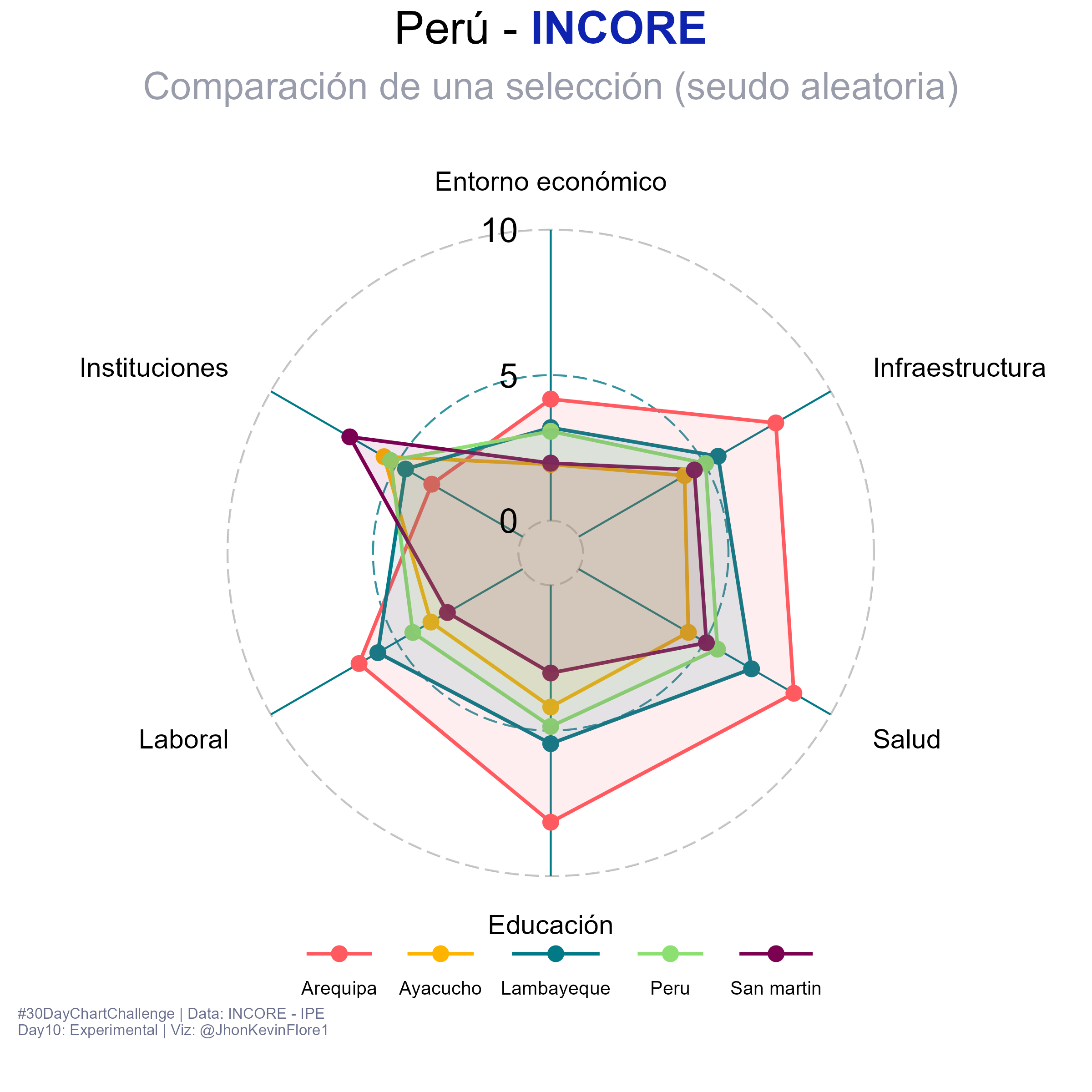
  select(edicion, pilar, region, valor, ano)

p <- 
  incor_2_gif |> 
  filter(ano == 2021) |> 
  select(!ano) |> 
  select(!edicion) |> 
  pivot_wider(names_from = pilar, values_from = valor) |> 
  # mutate_at(vars(!region), rescale) |> 
  # janitor::clean_names() |> 
  ggradar::ggradar(
    grid.max = 10
    , grid.mid = 5
    , grid.line.width = .5
    , grid.label.size = 8
    , group.point.size = 3.5
    , group.line.width = 0.9
    , base.size = 20
    , values.radar = c(0, 5, 10)
    , axis.line.colour = "#007A87"
    , background.circle.colour = "white"
    # , legend.position = c(.1, .1)
    , fill = T
    , fill.alpha = .1
    , legend.text.size = 10
  ) +
  labs(
    title = 'Perú - <span style="color:#0e23af">**INCORE**</span>'
    , subtitle = "Comparación de una selección (seudo aleatoria)"
    , caption = "#30DayChartChallenge | Data: INCORE - IPE\nDay10: Experimental | Viz: @JhonKevinFlore1"
  ) +
  guides(
    colour = guide_legend(label.position = "bottom")
    , fill = NULL
    ) +
  theme(
    panel.background = element_rect("white", color = NA)
    , plot.background = element_rect("white")
    , legend.background = element_rect(NA)
    , legend.key = element_rect(NA)
    , legend.spacing.y = unit(0, "lines")
    , legend.text = element_text(lineheight = 0, margin = margin(0, 0, 0, 0))
    # , legend.spacing = 
    , legend.margin = margin(c(0, 0, 0, 0))
    , plot.title = element_markdown(hjust = .5)
    , plot.subtitle = element_text(hjust = .5, color = "#999caa")
    , plot.margin = margin(.2, 0, 1, 0, unit = "cm")
    , plot.caption = element_text(size = 8, hjust = 0, color = "#696e8e") 
    , plot.caption.position = "panel"
    # , legend.position = "top"
    , legend.direction = "horizontal"
    , legend.position = c(.5, .02)
  )

ggsave(
  'plots/day10_dcc_22.png'
  , plot = p
  , height = 8 
  , width = 8
)

knitr::include_graphics('plots/day10_dcc_22.png')