Day 13

Day 13 from #30dataChartChallenge

librarian::shelf(
  tidyverse
  , cowplot
)

gdp_ene <- 
  read_csv(
  here::here(
    "data", "owd", "electr-gpr.csv"
  )
) |> 
  janitor::clean_names() |> 
  filter(year %in% 2019) |> 
  rename(acces = 4, gdp = 5, pop = 6) |> 
  drop_na(acces, gdp) |> 
  mutate(
    acces = acces / 100
  )
  


options(scipen = 999)

p1 <- 
  gdp_ene |> 
  ggplot() +
  aes(gdp, acces, size = pop) +
  geom_point() +
  # geom_smooth(se = F) +
  scale_size(range(7, 6)) +
  theme_bw() +
  labs(
    x = "PIB per capita"
    , y = "Acceso a la electricidad"
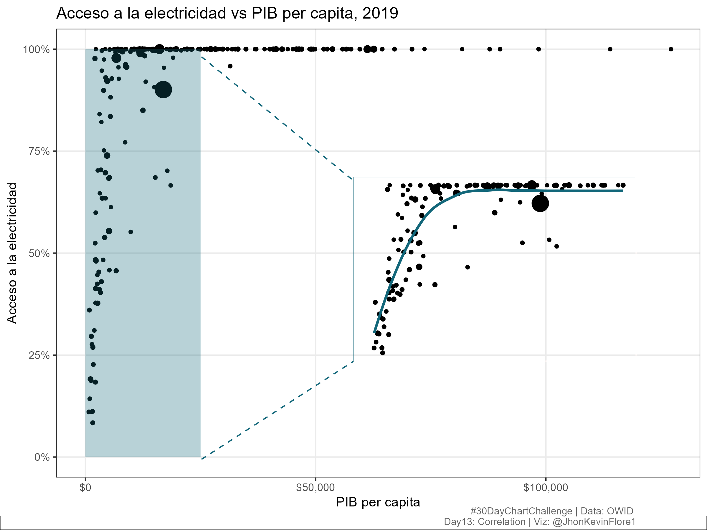
    , title = "Acceso a la electricidad vs PIB per capita, 2019"
  ) +
  scale_y_continuous(labels = scales::percent) +
  scale_x_continuous(labels = scales::dollar) +
  theme(
    legend.position = "none"
    , panel.grid.minor = element_blank()
  )

f_c <- "#12677a"
p3 <- 
  p1 +
  annotate(
    "rect"
    , xmin = 0, xmax = 25000
    , ymin = 0, ymax = 1
    , alpha = .3
    , fill = f_c
  ) 

p2 <- 
  p1 +
  scale_x_continuous(
    labels = scales::dollar, limits = c(0, 25000)
    , breaks = seq(0, 25000, by = 8000)
    ) +
  geom_smooth(se = F, color = f_c) +
  labs(
    title = ""
    , y = ""
    , x = ""
    ) +
  theme_void() +
  theme(
    legend.position = "none"
    ,  panel.background = element_rect(NA, color = f_c)
  )

p <- 
  ggdraw(p3) +
  draw_plot(
    p2, height = .4, width = .4
    , x = .5
    , y = .3
    )

p +
  draw_line(
    x = c(.285, .5)
    , y = c(.11, .3)
    , linetype = "dashed"
    , color = f_c
  ) +
  draw_line(
    x = c(.285, .5)
    , y = c(.89, .65)
    , linetype = "dashed"
    , color = f_c
  ) +
  theme(
    plot.margin = margin(0, 0, .4, 0, "cm")
    , plot.background = element_rect("white")
  ) +
  draw_label(
    "#30DayChartChallenge | Data: OWID \nDay13: Correlation | Viz: @JhonKevinFlore1"
    , x = .9
    , y = 0
    , color = "grey40"
    , size = 8
    , hjust = 1
  )


ggsave(
  'plots/day13_dcc_22.png'
  # , plot = p
  , width = 8
  , height = 6
)

knitr::include_graphics('plots/day13_dcc_22.png')