Day 16

Day 16 from #30dataChartChallenge

zona <- 
  read_rds(here::here("data", "zonas.rds"))

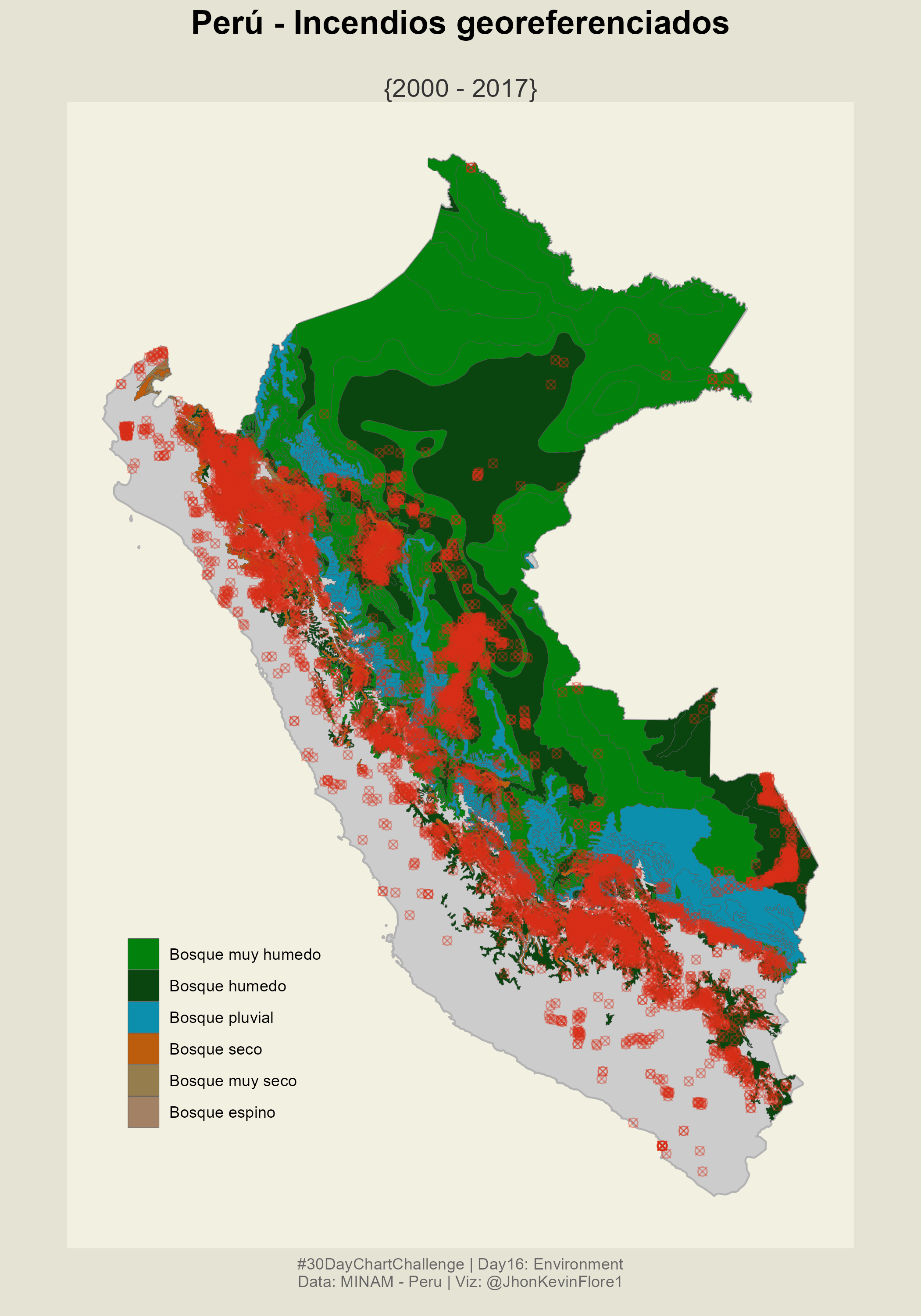
h_inc <- 
  dir(recursive = T, pattern = "shp$", full.names = T) |> 
  read_sf() |> 
  janitor::clean_names()

orden <- 
  zona |> 
  # st_drop_geometry() |> 
  select(tipo, sum_km2) |> 
  with_groups(tipo, summarise, t = sum(sum_km2)) |> 
  pull(tipo)

colores <- 
  c(
     "#02820d"
    , "#0a440f"
    , "#0c8fad"
    , "#bc5c0d"
    , "#967d4e"
    , "#a38165"
  )



zona1 <- 
  zona |> 
  mutate(tipo = factor(tipo, orden))

rango <- c(min(h_inc$ano), max(h_inc$ano))
  
p <- 
  zona1 |> 
  select(tipo, geometry) |> 
  st_as_sf() |> 
  ggplot()+
  geom_sf(data = map_peru_peru, fill = "grey80", color = "grey70") +
  geom_sf(aes(fill = tipo), size = .1) +
  scale_fill_manual(values = colores) +
  labs(
    fill = ""
    , title = "Perú - Incendios georeferenciados"
    , subtitle = " \n{2000 - 2017}"
    , caption = "#30DayChartChallenge | Day16: Environment\nData: MINAM - Peru | Viz: @JhonKevinFlore1"
    ) +
  geom_sf(data = h_inc, shape = 13, color = "#d82e17", alpha = .4, size = 2)  +
  theme_void() +
  theme(
    panel.background = element_rect("#f2f0e1", color = NA)
    , plot.background = element_rect("#e5e3d3", color = NA)
    , plot.caption = element_text(hjust = .5, color = "gray40")
    , plot.title = element_text(hjust = .5, size = 18, face = "bold")
    , plot.subtitle = element_text(hjust = .5, size = 14, color = "gray20")
    , legend.position = c(.2, .2)
    , plot.margin = margin(0, 0, 0.5, 0, "cm")
  )

ggsave(
  'plots/day16_dcc_22.png'
  , plot = p
  , width = 7
  , height =10
)

knitr::include_graphics('plots/day16_dcc_22.png')