Day 17

Day 17 from #30dataChartChallenge

librarian::shelf(
  tidyverse
  , PeruData
  , sf
)

cuencas <- read_rds(here::here("data", "cuencas.rds")) |> 
  janitor::clean_names()


# unique(cuencas$nomb_uh_n2)
rh <- unique(cuencas$nomb_uh_n1) |>   str_sub(25, -1) 
rh <- paste("R.H. del\n", rh)
names(rh) <- c(
  "#659dce"
  , "#0e9e04"
  , "#cc5612"
  )
cl <- "grey90"


cuencas$nomb_uh_n1 <- factor(cuencas$nomb_uh_n1, unique(cuencas$nomb_uh_n1))

knitr::include_graphics('plots/day17_dcc_22.png')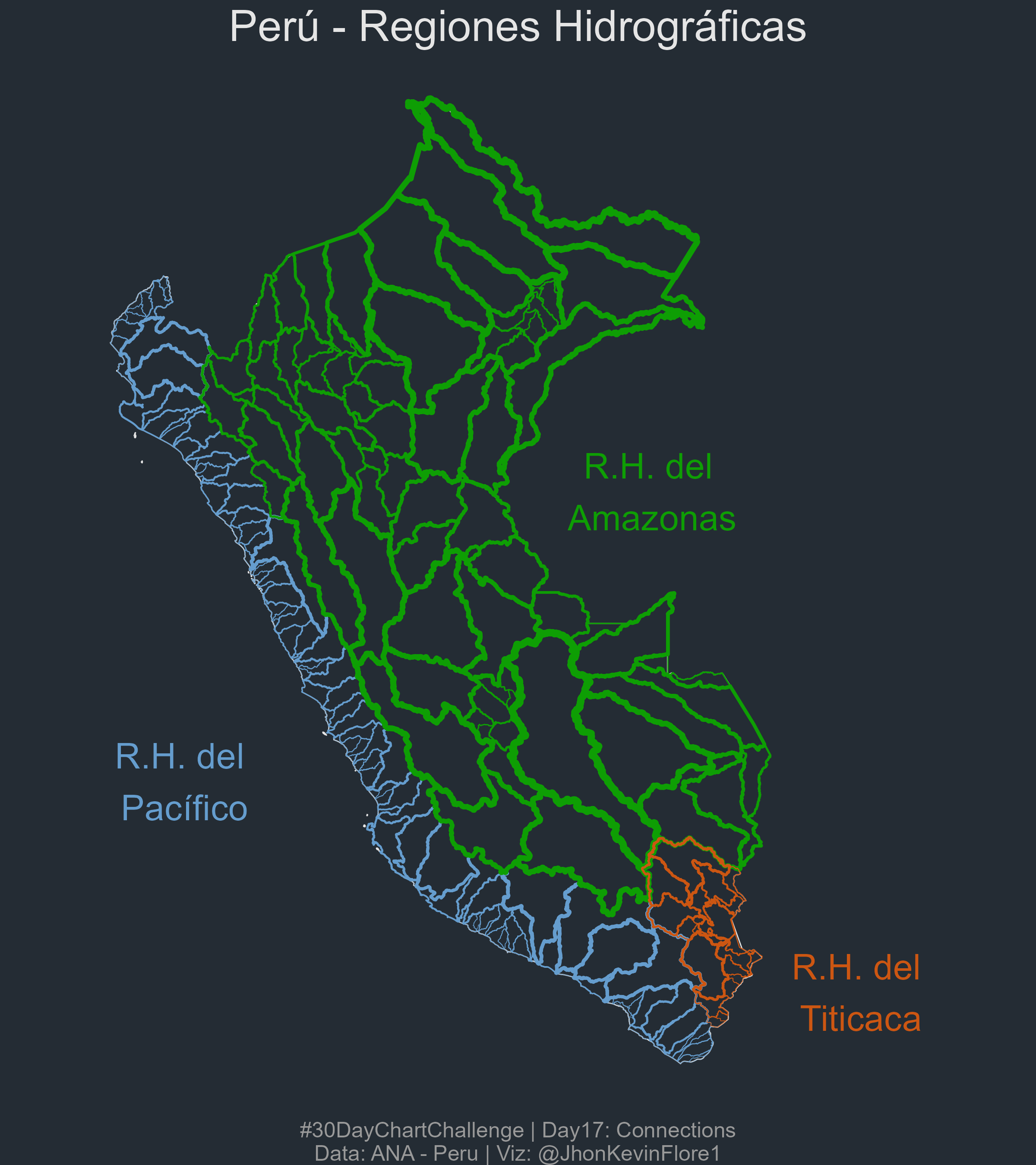

p <- 
  ggplot() +
  geom_sf(data = map_peru_peru, fill = NA, color = cl, size = .3, alpha = .1) +
  geom_sf(data = cuencas, aes(color = nomb_uh_n1, size = area_km2), alpha = .2, fill = NA) +
  scale_size(range = c(0, 1.8)) +
  labs(
    title = "Perú - Regiones Hidrográficas"
    , caption = "#30DayChartChallenge | Day17: Connections\nData: ANA - Peru | Viz: @JhonKevinFlore1"
  ) +
  scale_color_manual(values = names(rh)) +
  annotate("text", x = -80, y = -13, label = rh[1], color = names(rh)[1], size = 7) +
  annotate("text", x = -71, y = -7.5, label = rh[2], color = names(rh)[2], size = 7) +
  annotate("text", x = -67, y = -17, label = rh[3], color = names(rh)[3], size = 7) +
  xlim(-82, -65) +
  theme_void() +
  theme(
    legend.position = "none"
    , plot.title = element_text(hjust = .5, size = 24, color = cl)
    , plot.caption = element_text(hjust = .5, size = 12, color = "grey60")
    # , plot.background = element_blank()
    # , plot.margin = margin(1,10, 1, 1, "in")
    # , panel.border = margin(1, 1, 1, 1, "in")
  ) 

ggsave(
  here::here("plots", "day17_temp.png")
  , plot = p
  , height = 9
  , width = 8
  , scale = 1
  , bg = "#242c34"
  # , unit = "px"
  # , units = "cm"
)

amz <- cuencas |> filter(str_detect(nomb_uh_n2, "Amazonas"))
amz_sub <-
  amz |>
  sf::st_drop_geometry() |>
  count(nomb_uh_n3, sort = T) |>
  add_column(color = c_color)

amz_cuencas <-
  ggplot() +
  geom_sf(data =  map_peru_peru, color = "white", fill = NA, size = .2) +
  geom_sf(data = amz, aes(size = area_km2, group = nomb_uh_n3, color = nomb_uh_n3), fill = NA) +
  scale_size(range = c(0, 1.3)) +
  scale_color_manual(values = pull(amz_sub, color)) +
  theme_void()

amz_cuencas1 <- amz_cuencas +
  theme(legend.position = "none")

lab_c <- pull(amz_sub, nomb_uh_n3)
lab_c[3] <- "U.H. 497"

ggdraw(xlim = c(0, 1), ylim = c(0, 1))  +
  draw_plot(amz_cuencas1, x = -.2) +
  theme(
    plot.background = element_rect(fill = "#242c34")
  ) +
  draw_label(label = lab_c[3], x = 0.55, y = 0.85, color = c_color[4], fontfamily = font1,hjust = 0, fontface = "bold", size = 55) +
  draw_label(label = lab_c[1], x = 0.55, y = 0.79, color = c_color[1], fontfamily = font1,hjust = 0, fontface = "bold", size = 55) +    # draw_label(label = lab_c[1], x = 0.55, y = 0.85, color = c_color[1], fontfamily = font1,hjust = 0, fontface = "bold", size = 55) +
  draw_label(label = lab_c[2], x = 0.55, y = 0.73, color = c_color[3], fontfamily = font1,hjust = 0, fontface = "bold", size = 55) +
  draw_label(label = lab_c[4], x = 0.55, y = 0.6169, color = c_color[2], fontfamily = font1,hjust = 0, fontface = "bold", size = 55) +
  draw_label(label = lab_c[5], x = 0.55, y = 0.67, color = c_color[5], fontfamily = font1,hjust = 0, fontface = "bold", size = 55) +
  draw_label(
    label = "Cuencas hidrograficas del Perú (UH Amazonas)\n#30DayMapChallenge | Day 2: Lines\nData: ANA | Created by @JhonKevinFlore1"
    , lineheight = .3
    , color = "white"
    , x = .92
    , y = .08
    , hjust = 1
    , fontfamily = font1
  )

ggsave('plots/day17_dcc_22.png', units = "cm", width = 9.6, height = 8.73)

knitr::include_graphics('plots/day17_dcc_22.png')