Day 01

Day 2 form #30datChartChallenge

#load libraries
librarian::shelf(
  tidyverse
  , showtext
  , ggtext
  , sysfonts
  , emojifont
  , cowplot
)

caritas <- 18
b <- "grey60"
p_d <- "#df4576"
s_d <- "#238ad3"
t_d <- "#27eBa7"


vacc <-
  PeruData::covid_estado_situacional("04/02/2022") |> 
  mutate(
    d11 = d1 / 32781250
    , d21 = d2 / d1
    , d31 = d3 / d2
  ) |> 
  gather() |> 
  slice(4:6) |> 
  mutate(
    count = as.integer(value * caritas)
    , total = list(1:caritas)
    )  |> 
  unnest(total) |> 
  rename(
    dosis = 1
    , percet = 2
  ) |> 
  mutate(
    dosis = as.numeric(str_sub(dosis, 2, 2))
    , color = case_when(
      dosis == 1 & total < count  ~ p_d
      , dosis == 2 & total < count ~ s_d
      , dosis ==3 & total< count ~ t_d
      , T ~ b
    )
    , poss = case_when(
      dosis == 1 ~ 2
      , dosis == 3 ~ 1
      , T ~ 1.5
    )
  ) 
p <- vacc |> 
  ggplot() +
  geom_text(
    aes(
      x = total,
      y = poss,
      color = color,
      label = emoji("busts_in_silhouette")
    ),
    family = "EmojiOne",
    size = 30
  ) +
  scale_color_identity() +
  ylim(0.2, 2) +
  xlim(-2, 18) +
  labs(
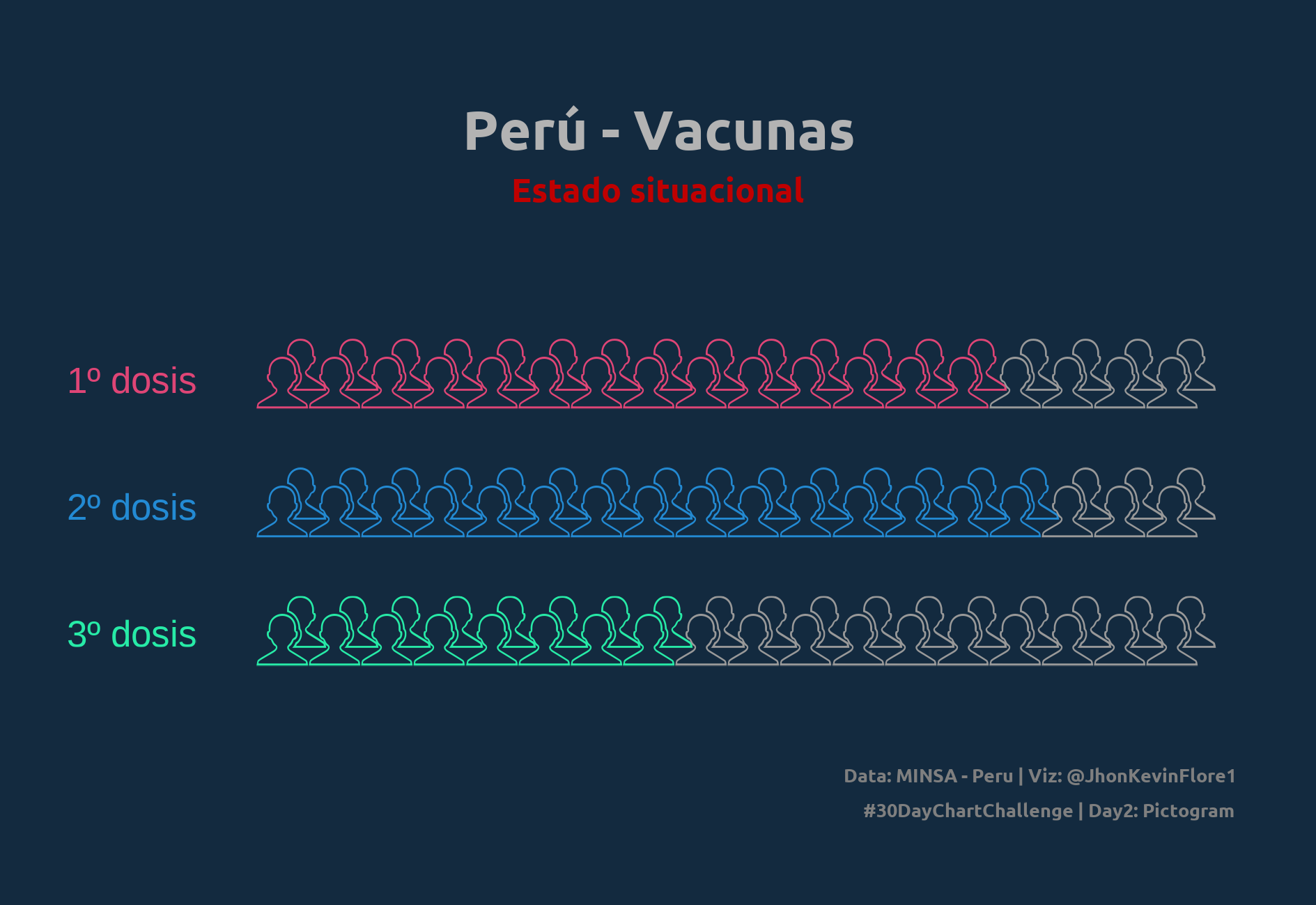
    title = "Perú - Vacunas"
    , caption = "Data: MINSA - Peru | Viz: @JhonKevinFlore1\n#30DayChartChallenge | Day2: Pictogram"
    , subtitle = "Estado situacional"
    ) +
  theme_void() +
  theme(
    text = element_text(
      family = "Ubuntu",
      face = 'bold',
      colour = "#004D40"
    ),
    plot.background = element_rect(fill = "#132A3F", color = NA),
    plot.title = element_text(
      hjust = 0.5,
      size = 60,
      margin = margin(10, 0, 0, 0),
      color = "grey70"
    ),
    plot.subtitle = element_text(
      hjust = 0.5,
      size = 36,
      margin = margin(10, 0, 0, 0),
      color = "#c00000"
    ),
    plot.caption = element_text(
      hjust = 1,
      margin = margin(20, 0, 2, 0),
      color = "grey50"
      , lineheight = .5
      , size = 20
    ),
    plot.margin = margin(1, 1, 1, 1, unit = "cm")
  )


ggdraw() +
  draw_plot(p) +
  draw_label("1º dosis", x = .1, y = .58, size = 40, color = "#df4576") +
  draw_label("2º dosis", x = .1, y = .44, size = 40, color = "#238ad3") +
  draw_label("3º dosis", x = .1, y = .3, size = 40, color = "#27eBa7")

# ggsave(
  # , width = 16, height = 11, units = "cm") 

knitr::include_graphics('plots/day2_dcc_22.png')