Day 05

Day 5 form #30dataChartChallenge

p_name = 'plots/day5_dcc_22.png'
knitr::opts_chunk$set(
  eval = F
)

librarian::shelf(
  tidyverse
  , PeruData
  , ggtext
)

# Enaho, P524A1 ingresos
# p207 sexo
# p510 ocupacion principal para
# 
# 

vari <- c("p524a1", "p207", "p510")

#data

# PeruData::inei_enaho("05", c("2010", "2020"))

enaho <- dir(here::here("Data", "enaho", "solo-data"), recursive = T, pattern = ".dta", full.names = T)

semi_clean <- function(dir){
  enaho <- 
    haven::read_dta(dir) |> 
    janitor::clean_names()
  Sys.sleep(5)
  variables <- 
    enaho |> 
    select(any_of(vari)) |> 
    rename(ing = 1, sex = 2, ocu = 3) |> 
    drop_na() |> 
    group_by(ocu, sex) |> 
    summarise(ing_mean = mean(ing), n = n())
  Sys.sleep(5)
  return(variables)
}

enaho_data <- 
  map(enaho, semi_clean) |> 
  map_dfr(ungroup, .id = "anio") |> 
  mutate(
    anio = ifelse(anio == 1, 2010, 2020)
    , sex = ifelse(sex ==1, "Hombre", "Mujer")
  )

bg <- "#132A3F"

enaho_data |> 
  mutate(
    ocu = haven::as_factor(ocu)
    # , anio = factor(anio, c(2010, 2020))
    , n_per = BBmisc::normalize(n, "range", c(1, 3))
  ) |> 
  filter(ocu != "Cooperativa de trabajadores") |> 
  
  ggplot() +
  aes(
    anio, ing_mean, group = interaction(ocu, sex), color = sex, linetype = ocu, shape = sex
      ) +
  ggtitle(
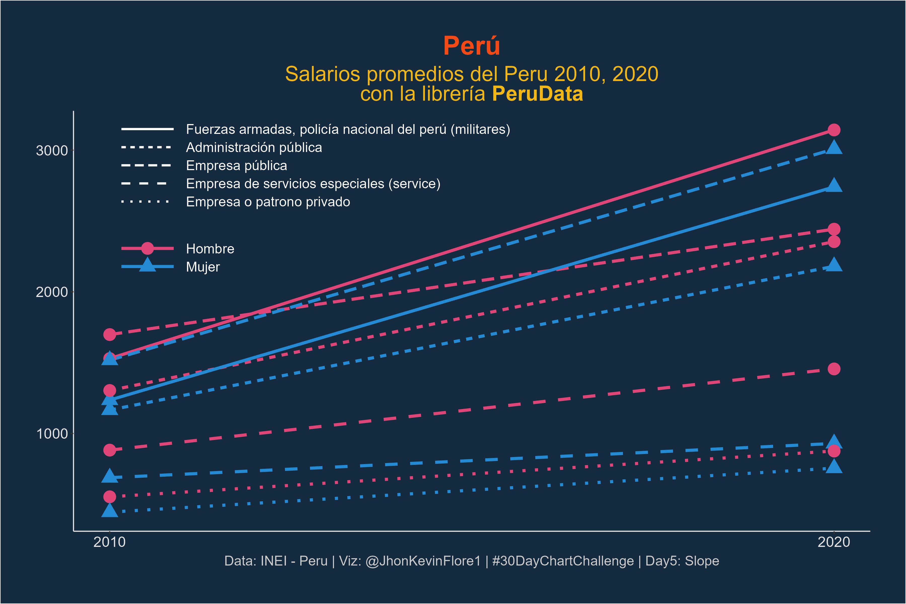
    "Perú"
    , subtitle = glue::glue("Salarios promedios del Peru 2010, 2020<br> con la librería **PeruData**")
  ) +
  labs(
     caption = "Data: INEI - Peru | Viz: @JhonKevinFlore1 | #30DayChartChallenge | Day5: Slope"
    
  ) +
  scale_color_manual(values = c("#df4576", "#238ad3")) +
  geom_line(size = 1.4)  +
  geom_point(size = 5.4) +
  scale_x_continuous(breaks = c(2010, 2020)) +
  guides(
    linetype = guide_legend(
      override.aes = list(
        color = "white"
        , size = 1
        )
    )
  ) +
  theme(
    plot.background = element_rect(bg)
    , panel.background = element_rect(bg)
    , axis.text = element_text(color = "grey90", size = 14)
    , axis.line = element_line(color = "grey90") 
    , axis.title = element_blank()
    , panel.grid = element_blank()
    , legend.background = element_rect(NA)
    , legend.key = element_rect(NA, color = bg)
    , legend.text = element_text(color ="white", size = 13)
    , legend.key.width = unit(22, "mm")
    , legend.title = element_blank()
  
    , legend.position = c(.3, .8)
    , plot.title = element_text(
      hjust = .5, color = "#f24915"
      , size = 25, face = "bold"
      )
    # , plot.subtitle = element_text(
    #   hjust = .5, color = "#f2b715"
    #   , size = 20
    # 
    # )
    , plot.subtitle = element_markdown(
      hjust = .5, color = "#f2b715"
      , size = 20
    )
    , plot.caption = element_text(
      hjust = .5, color = "grey80"
      , size = 13
      , 
    )
    , plot.margin = unit(rep(12, 4), "mm")
  )  

ggsave(
  height = 8 
  , width = 12
  , filename = "plots/day5_dcc_22.png"

)

knitr::include_graphics('plots/day5_dcc_22.png')