librarian::shelf(
  tidyverse
  , ggtext
  , tidytuesdayR
  , ggside
)
  The 'cran_repo' argument in shelf() was not set, so it will use
  cran_repo = 'https://cran.r-project.org' by default.

  To avoid this message, set the 'cran_repo' argument to a CRAN
  mirror URL (see https://cran.r-project.org/mirrors.html) or set
  'quiet = TRUE'.
Warning: package 'ggtext' was built under R version 4.3.1Warning: package 'tidytuesdayR' was built under R version 4.3.1Warning: package 'ggside' was built under R version 4.3.1# tt_available()
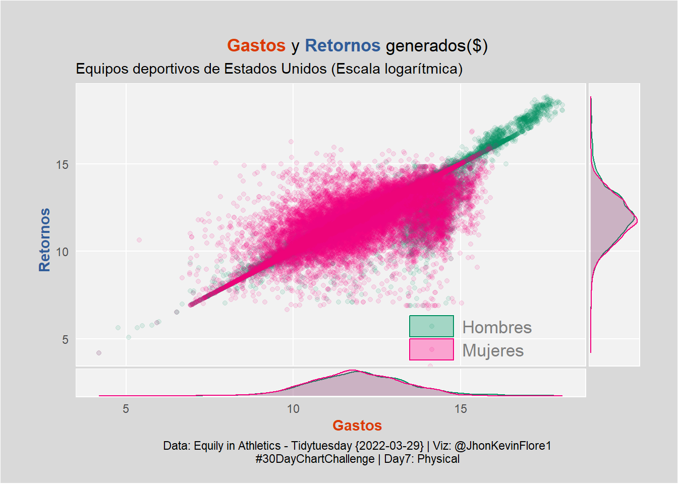
tt <- tt_load("2022-03-29")--- Compiling #TidyTuesday Information for 2022-03-29 ------- There is 1 file available ------ Starting Download ---
Downloading file 1 of 1: `sports.csv`--- Download complete ---sports <- tt$sports
glimpse(sports)Rows: 132,327
Columns: 28
$ year <dbl> 2015, 2015, 2015, 2015, 2015, 2015, 2015, 2015, 2…
$ unitid <dbl> 100654, 100654, 100654, 100654, 100654, 100654, 1…
$ institution_name <chr> "Alabama A & M University", "Alabama A & M Univer…
$ city_txt <chr> "Normal", "Normal", "Normal", "Normal", "Normal",…
$ state_cd <chr> "AL", "AL", "AL", "AL", "AL", "AL", "AL", "AL", "…
$ zip_text <chr> "35762", "35762", "35762", "35762", "35762", "357…
$ classification_code <dbl> 2, 2, 2, 2, 2, 2, 2, 2, 2, 2, 1, 1, 1, 1, 1, 1, 1…
$ classification_name <chr> "NCAA Division I-FCS", "NCAA Division I-FCS", "NC…
$ classification_other <chr> NA, NA, NA, NA, NA, NA, NA, NA, NA, NA, NA, NA, N…
$ ef_male_count <dbl> 1923, 1923, 1923, 1923, 1923, 1923, 1923, 1923, 1…
$ ef_female_count <dbl> 2300, 2300, 2300, 2300, 2300, 2300, 2300, 2300, 2…
$ ef_total_count <dbl> 4223, 4223, 4223, 4223, 4223, 4223, 4223, 4223, 4…
$ sector_cd <dbl> 1, 1, 1, 1, 1, 1, 1, 1, 1, 1, 1, 1, 1, 1, 1, 1, 1…
$ sector_name <chr> "Public, 4-year or above", "Public, 4-year or abo…
$ sportscode <dbl> 1, 2, 3, 7, 8, 15, 16, 22, 26, 33, 1, 2, 3, 8, 12…
$ partic_men <dbl> 31, 19, 61, 99, 9, NA, NA, 7, NA, NA, 32, 13, NA,…
$ partic_women <dbl> NA, 16, 46, NA, NA, 21, 25, 10, 16, 9, NA, 20, 68…
$ partic_coed_men <dbl> NA, NA, NA, NA, NA, NA, NA, NA, NA, NA, NA, NA, N…
$ partic_coed_women <dbl> NA, NA, NA, NA, NA, NA, NA, NA, NA, NA, NA, NA, N…
$ sum_partic_men <dbl> 31, 19, 61, 99, 9, 0, 0, 7, 0, 0, 32, 13, 0, 10, …
$ sum_partic_women <dbl> 0, 16, 46, 0, 0, 21, 25, 10, 16, 9, 0, 20, 68, 7,…
$ rev_men <dbl> 345592, 1211095, 183333, 2808949, 78270, NA, NA, …
$ rev_women <dbl> NA, 748833, 315574, NA, NA, 410717, 298164, 13114…
$ total_rev_menwomen <dbl> 345592, 1959928, 498907, 2808949, 78270, 410717, …
$ exp_men <dbl> 397818, 817868, 246949, 3059353, 83913, NA, NA, 9…
$ exp_women <dbl> NA, 742460, 251184, NA, NA, 432648, 340259, 11388…
$ total_exp_menwomen <dbl> 397818, 1560328, 498133, 3059353, 83913, 432648, …
$ sports <chr> "Baseball", "Basketball", "All Track Combined", "…unique(sports$sports) [1] "Baseball" "Basketball"
[3] "All Track Combined" "Football"
[5] "Golf" "Soccer"
[7] "Softball" "Tennis"
[9] "Volleyball" "Bowling"
[11] "Rifle" "Beach Volleyball"
[13] "Ice Hockey" "Lacrosse"
[15] "Gymnastics" "Rowing"
[17] "Swimming and Diving" "Track and Field, X-Country"
[19] "Equestrian" "Track and Field, Indoor"
[21] "Track and Field, Outdoor" "Wrestling"
[23] "Other Sports" "Rodeo"
[25] "Skiing" "Swimming"
[27] "Water Polo" "Archery"
[29] "Field Hockey" "Fencing"
[31] "Sailing" "Badminton"
[33] "Squash" "Diving"
[35] "Synchronized Swimming" "Table Tennis"
[37] "Weight Lifting" "Team Handball"