Day 08

Day 8 from #30dataChartChallenge

librarian::shelf(
  ggridges
  , tidyverse
  , PeruData
  , sf
  , raster
  , cowplot
)

peru <- 
  raster_peru_alt |> 
  mask(map_peru_depa) |> 
  rasterToPoints() |> 
  as_tibble() |> 
  rename(alt = 3)

depas <- 
  unique(map_peru_depa$depa)


get_alt <- function(dep){
  depa <- 
    map_peru_depa |> 
    filter(depa == dep)
  alt <- 
    raster_peru_alt |> 
    mask(depa) |> 
    rasterToPoints() |> 
    as_tibble() |> 
    rename(alt = 3)
  return(alt)
}

sierra_map <- 
  map(depas, get_alt)

names(sierra_map) <- depas

peru_alt <- 
  bind_rows(sierra_map, .id = "depa")

alt_cl <- colorRampPalette(c("#e5e4d3", "#3f2a04"))

p <- 
  ggplot() +
  geom_tile(data = peru_alt, aes(x, y, fill = alt)) +
  geom_sf(data = map_peru_depa, aes(geometry = geometry), fill = NA, size = .5, color = "grey45") +
  scale_fill_gradientn(colours = alt_cl(2)) +
  theme_void() +
  labs(
    fill = "M.S.N.M"
  ) +
  theme(
    legend.position = c(.2, .2)
    , legend.background = element_rect(color = "grey45")
    # , legend.box.margin = margin(1, 1, 110, 1, "pt")
    , legend.margin = margin(2, 3, 3, 5, "mm")
  )

levels_peru <- 
  peru_alt |> 
  group_by(depa) |> 
  # slice(1:200) |> 
  summarise(
    mean = mean(alt)
  ) |> 
  filter(depa != "callao") |> 
  arrange(mean) |> 
  pull(depa) |> 
  str_to_sentence()

p1 <- 
  peru_alt |> 
  filter(depa != "callao") |> 
  group_by(depa) |> 
  # slice(1:200) |> 
  mutate(
    mean = mean(alt)
    , depa = str_to_sentence(depa)
    , depa = factor(depa, levels = levels_peru)
    ) |> 
  ggplot() +
  aes(alt, str_to_sentence(depa), fill = ..x..) +
  # geom_density_ridges(
  #   # jittered_points = T
  #   position = position_points_jitter(width = .02, yoffset = .25, seed = 1)
  #   , alpha = .6
  # ) + 
  geom_density_ridges_gradient(
    scale = 3, alpha=.3
    , show.legend = F
    , color = "gray50"
    , size = .5
    # , seed
    ) +
  # viridis::scale_fill_viridis()
  scale_fill_gradientn(colours = alt_cl(2)) +
  theme_minimal() +
  labs(x = "", y = "")  +
  theme(
    panel.background = element_rect("white")
    , plot.background = element_rect("white")
  )
  
p3 <- 
  ggdraw(xlim = c(0, 4), ylim = c(0, 1)) +
  draw_plot(p, width = 1.2, x = .2) +
  draw_plot(p1, width = 2, height = .8, x = 1.7, y = .1) +
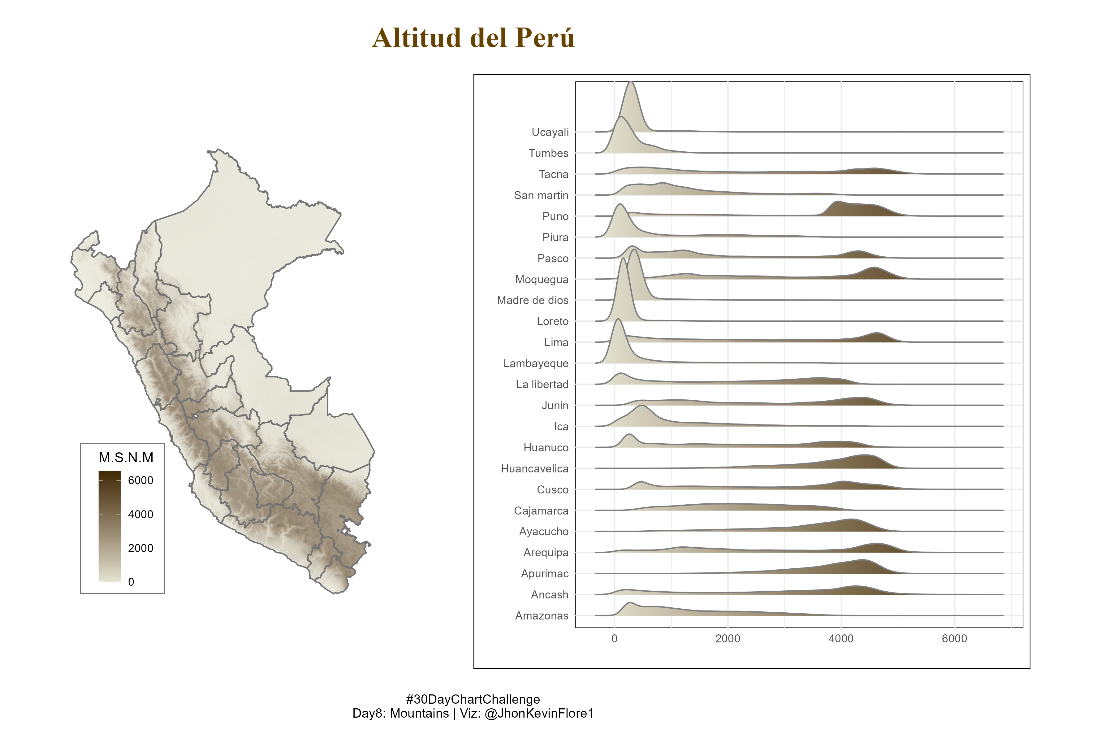
  draw_label(
    "Altitud del Perú"
    , hjust = .5
    , size = 23
    , x = 1.7
    , y = .95
    , fontface = "bold"
    , fontfamily = "serif"
    , color = "#664200"
    ) +
  draw_label(
    "#30DayChartChallenge\nDay8: Mountains | Viz: @JhonKevinFlore1"
    , x = 1.7
    , y = .05
    , hjust = .5
    , size = 10
    )

ggsave(
  'plots/day8_dcc_22.png'
  , plot = p3
  , height = 8
  , width = 12
  , bg = "white"
)

knitr::include_graphics('plots/day8_dcc_22.png')