Day 09

Day 9 from #30dataChartChallenge

librarian::shelf(
  tidyverse
  , PeruData
  , ggtext
)

# inei_endes("1638", "2020", "csv")
#

dir_endes <- 
  dir(here::here("data", "endes"), full.names = T)
endes2020 <- 
  read_csv2(dir_endes[2]) |> 
  janitor::clean_names() 

ed20 <-
  endes2020 |> 
  select(edad = ha1, kg = ha2, tll = ha3) |> 
  drop_na() |> 
  filter(kg != 9999) |> 
  arrange(-kg) |> 
  mutate(
    kg = kg / 10
    , tll = tll / 1000
    , rg_edad = cut_width(edad, 10)
    , imc = kg / (tll)^2
    , imc_lb = case_when(
      imc < 18.5 ~ "b"
      , imc > 30 ~ "t"
      , T ~ "m"
    )
  ) |>
  with_groups(rg_edad, mutate, m_imc = round(mean(imc), 1)) |> 
  filter(m_imc > 0)

# alt_cl <- colorRampPalette(c("#e5e4d3", "#3f2a04"))


p <- 
  ggplot(ed20) +
  aes(rg_edad, imc, group = rg_edad) +
  # geom_hline(yintercept = 18.5, color = "orange") +
  
  # geom_hline(yintercept = 18.6, color = "green") +
  # geom_hline(yintercept = 30, color = "green") +
  # geom_hline(yintercept = 30.3, color = "red") +

  geom_violin(size = 1.6, alpha = 2) +
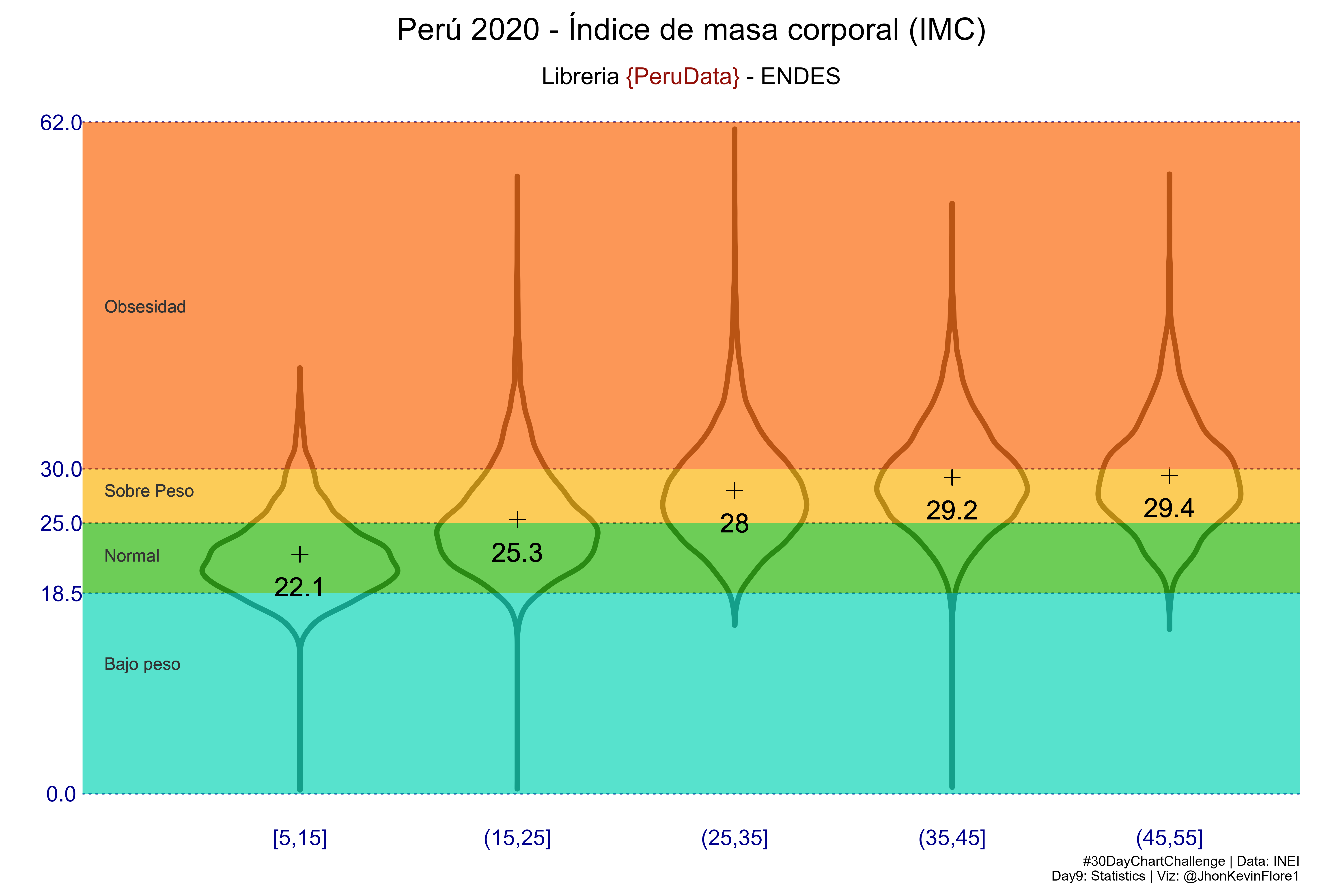
  ggtitle(
    "Perú 2020 - Índice de masa corporal (IMC)"
    , 'Libreria <span style="color:#930f08">{PeruData}</span> - ENDES'
  ) +
  scale_y_continuous(
    breaks = c(0, 18.5, 25, 30, 62)
  ) + 
  labs(
    caption = 
    "#30DayChartChallenge | Data: INEI\nDay9: Statistics | Viz: @JhonKevinFlore1"
    , x = ""
    , y = 'IMC'
  ) +
  annotate(
    "rect"
    , xmin = 0, xmax = 5.6
    , ymin = 0 , ymax = 18.5
    , alpha = .67
    , fill = "#04d4b4"
  ) + 
  annotate(
    "rect"
    , xmin = 0, xmax = 5.6
    , ymin = 18.51 , ymax = 25
    , alpha = .67
    , fill = "#25b405"
  ) +
  annotate(
    "rect"
    , xmin = 0, xmax = 5.6
    , ymin = 25 , ymax = 30
    , alpha = .67
    , fill = "#fbb306"
  ) +
  geom_point(aes(y = m_imc), size = 3, shape = 3, alpha = 3) +
  annotate(
    "rect"
    , xmin = 0, xmax = 5.6
    , ymin = 30 , ymax = 62
    , alpha = .67
    , fill = "#fb6405"
  ) +
  geom_text(
    aes(y = m_imc, label = m_imc)
    , size = 6
    , nudge_y = -3
  ) +
  geom_text(color = "gray20", hjust = 0, aes(x = 0.1, y = 12), label = "Bajo peso") +
  geom_text(color = "gray20", hjust = 0, aes(x = 0.1, y = 22), label = "Normal") +
  geom_text(color = "gray20", hjust = 0, aes(x = 0.1, y = 28), label = "Sobre Peso") +
  geom_text(color = "gray20", hjust = 0, aes(x = 0.1, y = 45), label = "Obsesidad") +
  theme_void() +
  theme(
    axis.title.y = element_text(hjust = .1, vjust = 3)
    , panel.grid.minor = element_blank()
    , panel.grid.major.x = element_blank()
    , panel.grid.major.y = element_line(
      color = "darkblue"
      , size = .5 
      , linetype = "dotted"
    )
    , axis.text = element_text(size = 14, color = "darkblue")
    , panel.background = element_rect("white", color = NA)
    , plot.background = element_rect("white", color = NA)
    , axis.line = element_blank()
    , plot.margin = margin(.2, 1, .3, .2, "cm")
    , plot.title = element_markdown(hjust = .5, size = 20)
    , plot.subtitle = element_markdown(hjust = .5, size = 15, margin = margin(.5, 0, 0, 0, "cm"))
  )

ggsave(
  'plots/day9_dcc_22.png'
  , plot = p
  , height = 8
  , width = 12  
  , dpi = 500
)

knitr::include_graphics('plots/day9_dcc_22.png')