knitr::include_graphics('plots/22-10-erasmus.png')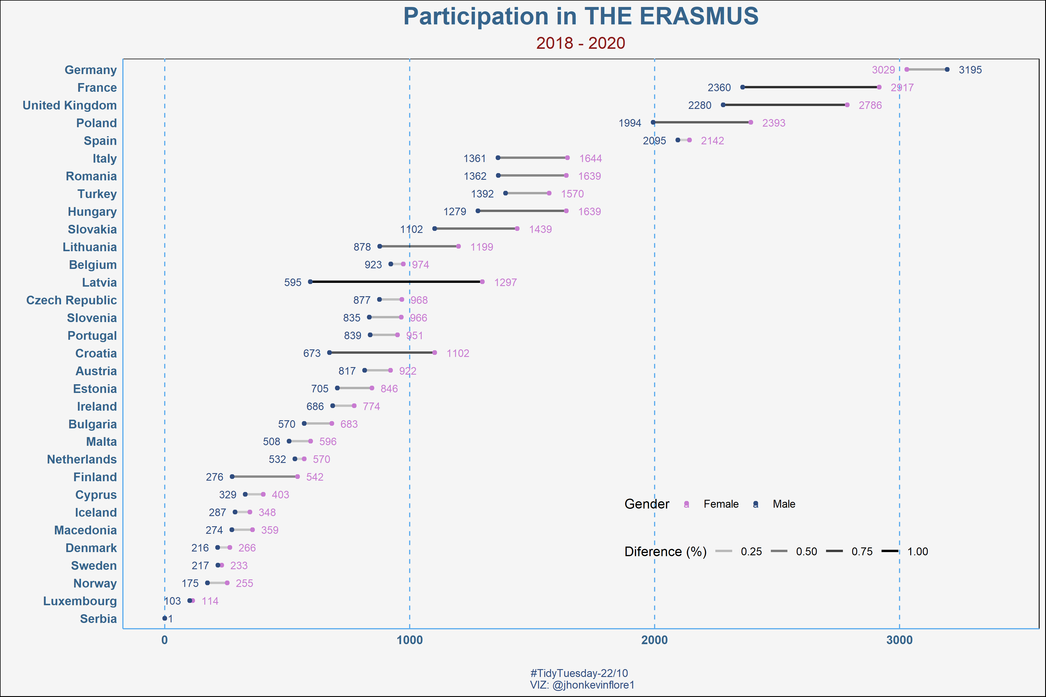
knitr::include_graphics('plots/22-10-erasmus.png')
librarian::shelf(
    tidyverse
    , tidytuesdayR
    , PeruData
)

tt <- tidytuesdayR::tt_load("2022-03-08")
erasmus <-
    tt$erasmus |>
    janitor::clean_names()

cc <- read_csv("https://gist.githubusercontent.com/tadast/8827699/raw/f5cac3d42d16b78348610fc4ec301e9234f82821/countries_codes_and_coordinates.csv") |>
    janitor::clean_names() |>
    select(1, 2) |>
    rename(code = 2)
country <-
erasmus |>
filter(
academic_year %in% c("2018-2019", "2019-2020")
) |>
select(
participant_nationality
, participant_gender
, participant_age
, receiving_country_code
, receiving_city
, activity_mob
) |> #uk
mutate(
across(
c(receiving_country_code, participant_nationality)
, ~ifelse(. == "UK", "GB", .)
)
) |>
count(
receiving_country_code, participant_gender
) |>
filter(participant_gender != "Undefined") |>
with_groups(1, ~mutate(., diff = max(n) - min(n), total = sum(n)), BSM) |>
mutate(diff_ap = BBmisc::normalize(diff, method = "range", range = c(.1, 1)))erasmus_20 <-
right_join(cc, country, by = c("code" = "receiving_country_code")) |>
drop_na(country) |>
mutate(
country = ifelse(str_detect(country, "Macedonia"), "Macedonia", country)
, country = forcats::fct_reorder(country, total))
erasmus_20
r_l <-
erasmus_20 |>
group_by(country) |>
arrange(desc(n)) |>
top_n(1, n)
l_l <-
erasmus_20 |>
group_by(country) |>
arrange(desc(n)) |>
slice(2)erasmus_20 |>
ggplot() +
aes(country, n) +
geom_line(aes(group = country, alpha = diff_ap), size = 1) +
geom_point(aes(color = participant_gender), size = 1.5) +
geom_text(
data = r_l
, aes(color = participant_gender, label = n)
, size = 3, hjust = -.5
) +
geom_text(
data = l_l
, aes(color = participant_gender, label = n)
, size = 3, hjust = 1.5
) +
ylim(0, 3400) +
scale_color_manual(values = c("#c87bd1", "#2f4c7f")) +
coord_flip() +
labs(
x = ""
, y = ""
, title = "Participation in THE ERASMUS"
, subtitle = "2018 - 2020"
, caption = "#TidyTuesday-22/10 \n VIZ: @jhonkevinflore1"
, alpha = "Diference (%)"
, color = "Gender"
) +
# theme_roboto()
theme_minimal() +
theme(
panel.background = element_rect(fill = "#F5F5F5"),
plot.background = element_rect(fill = "#F5F5F5"),
panel.grid = element_blank(),
panel.grid.major.x = element_line(color = "steelblue2", linetype = "dashed"),
plot.title = element_text(size = 20, hjust = .5, color = "steelblue4", face = "bold"),
plot.subtitle = element_text(size = 14, color = "firebrick4", hjust = 0.5),
plot.caption = element_text(color = "#2f4c7f", hjust=.5),
axis.line.x = element_line(color = "steelblue2", size = 0.5),
axis.line.y = element_line(color = "steelblue2", size = 0.5),
axis.text = element_text(size = 10, color = "steelblue4", face = "bold"),
axis.title = element_text(color = "steelblue4", face = "bold"),
# legend.title = element_blank(),
legend.justification = c(0, 1),
legend.position = c(.54, .25),
legend.background = element_blank(),
legend.direction="horizontal"
)
ggsave(here::here("plots/22-10-erasmus.png"), heigh=8, width = 12, unit='in')